
From Part L Failure to Compliance: Energy Modelling and Optimisation of a 12-Storey Office Building Using IES VE
A detailed case study of how I developed, simulated and iteratively optimised a 12-storey office building in IES VE, progressing from a substantial Part L 2021 failure to a compliant BER and BPER through lighting redesign, HVAC optimisation, airtightness, solar control and renewable energy integration.

Project Overview
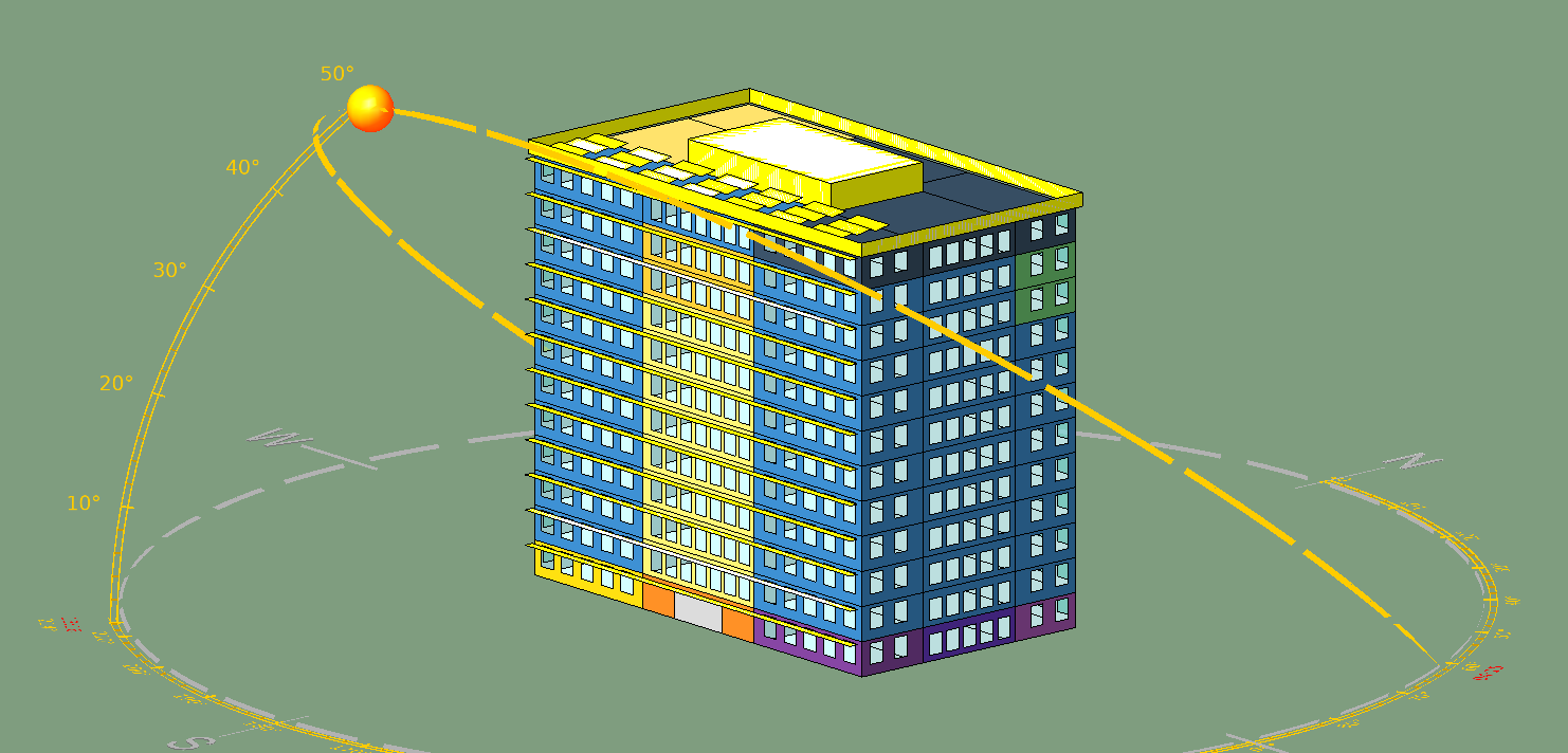
This project involved the energy modelling, building-services definition, performance analysis and Part L 2021 compliance assessment of a 12-storey office building in Birmingham, UK.
The final compliance model contained approximately 10,900.6 m² of floor area and was assessed as an office building using the Simplified Building Energy Model, SBEM v6.1.e.2, through the IES Virtual Environment compliance interface. The project was considerably more involved than simply creating geometry and clicking the compliance simulation button. It developed into an iterative building-performance exercise involving geometry, thermal zoning, constructions, internal gains, lighting design, HVAC systems, air permeability, solar gains, shading, domestic hot water, photovoltaics and solar thermal energy. The final model achieved the two principal Part L energy-performance requirements:
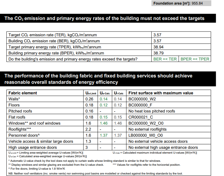
Part L metric | Actual building | Target/Notional | Final result | |
|---|---|---|---|---|
Building Emission Rate, BER | 3.57 kgCO₂/m²·yr | TER = 3.57 | PASS | |
Building Primary Energy Rate, BPER | 38.79 kWhPE/m²·yr | TPER = 38.94 | PASS |
The final BRUKL explicitly records both BER ≤ TER and BPER ≤ TPER.
What makes the project particularly useful as a building-performance case study is where it started.
The first compliance calculation produced:
BER = 7.07 against TER = 3.67
and:
BPER = 60.33 against TPER = 30.89
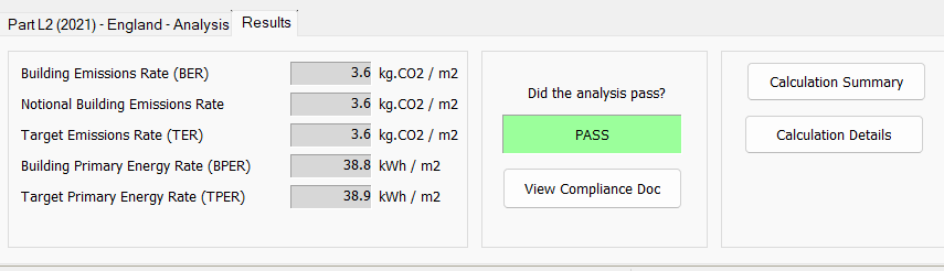
The building therefore failed both principal energy criteria by a very substantial margin.
Rather than attempting to force a pass by arbitrarily improving values, I used the failure as a diagnostic exercise and progressively rebuilt and optimised the model.
Building the Digital Model
The building originated from conventional project information including two-dimensional drawings and project data.
A major part of my workflow was reducing the amount of repetitive manual modelling normally required before a building can be analysed in IES VE. I developed an AI-assisted workflow to interpret the drawings and project brief and generate structured geometry suitable for transfer into the building-performance environment.
Individual spaces were identified and labelled consistently so that the resulting thermal zones could subsequently be mapped to appropriate activities, thermal templates and building-services assumptions.
I complemented this with Python-based automation for repetitive model-preparation work, including profile creation, room grouping and thermal-template assignment.
This was particularly valuable on a building of this scale. A 12-storey office contains repeated room types, circulation spaces, meeting rooms, open-plan offices, plant areas, WCs, lift cores, stairs and specialist spaces. Treating every space manually would not only be slow; it would increase the risk of inconsistent inputs between otherwise identical rooms. Automation therefore became part of the quality-control strategy rather than simply a time-saving measure.
Establishing the Initial Part L Baseline
The first SBEM/BRUKL run provided an excellent example of why a compliance result needs to be interrogated rather than treated simply as a pass/fail number. The initial model had a floor area of 10,900.6 m² and an air permeability of 10 m³/(h·m²) at 50 Pa, compared with 3 for the Notional Building.
The regulated end-use comparison was:
Energy end use | Initial actual | Initial notional | kWh/m²·yr |
|---|---|---|---|
Heating | 14.10 | 9.97 | High |
Cooling | 0.00 | 0.00 | Incomplete system representation |
Auxiliary | 2.02 | 1.01 | Low, but not representative of the later HVAC design |
Lighting | 27.32 | 9.68 | Major problem |
Hot water | 3.52 | 1.95 | High |
Total regulated energy | 43.16 | 22.61 | Major gap |
The initial result therefore could not be addressed by one intervention. There were problems with both building performance and model definition. For example, the early BRUKL described the HVAC arrangement as central heating through water radiators with an ASHP and did not represent the later cooling arrangement. There was also a CHP generator appearing in the early calculation, while no PV or solar thermal contribution was recognised. My first task was therefore not to optimise the building. It was to make sure I was optimising the correct building.
Using the BRUKL as a Diagnostic Tool
I adopted a controlled iterative approach. Rather than changing five or ten parameters between calculations, I progressively isolated the major contributors, changed one design area at a time, reran the compliance calculation and compared the Actual and Notional Buildings again. This was important because the Notional Building is not simply a fixed benchmark that remains unchanged regardless of the model. As the actual building and servicing strategy became properly defined, the target performance also changed. Consequently, I avoided the temptation to judge progress only by whether BPER or BER had fallen. Each result had to be assessed against its contemporaneous TER and TPER. Several areas emerged as particularly important.
Lighting: The First Major Performance Problem
Lighting was one of the clearest problems in the original model.
The Part L report used a general luminaire efficacy benchmark of 95 lm/W, yet many of the initial zones were reporting only around 24–35 lm/W. Open-plan offices and meeting rooms were typically around 24–25 lm/W.
This was consistent with an outdated fluorescent-lighting assumption rather than a modern commercial LED installation.
I therefore reviewed the lighting methodology rather than simply reducing an internal-gain number.
The model was moved toward a full-design lighting approach, with realistic design illuminance, installed wattage and control assumptions. Repeated office types were handled consistently while allowing different total wattages according to room area rather than applying one arbitrary wattage everywhere.
The resulting improvement was substantial.
By the final calculation, typical office lighting efficacy had increased to around 110 lm/W, with several zones considerably higher depending on their configuration. Meeting rooms were around 116 lm/W, while some other spaces achieved higher reported efficacies.
Whole-building lighting energy ultimately fell from:
27.32→6.84 kWh/m²\yr
a reduction of approximately 75%.
The final building actually performed substantially better than the Notional Building for lighting:
6.84 vs 9.68 kWh/m²\yr
This was one of the strongest improvements in the entire project.
Rebuilding the HVAC Strategy
The initial compliance model did not adequately represent the servicing strategy required for a modern multi-storey office.
The HVAC model therefore evolved into a mechanically ventilated office system incorporating a central air-handling strategy and fan-coil terminal units, with an ASHP-based heating system and electric cooling.
The final BRUKL identifies the HVAC system as AHU_VAV_ASHP and reports:
HVAC parameter | Final value |
|---|---|
Heating efficiency | 4.5 |
Cooling efficiency | 4.5 |
Central system SFP | 1.50 W/(L/s) |
Heat recovery efficiency | 76% |
Fan-coil terminal SFP | 0.30 W/(L/s) |
This stage required considerably more investigation than simply selecting an HVAC system from a drop-down menu.
Heating source, cooling generator, generator capacity, seasonal EER, nominal EER, ventilation, fan power, heat recovery, controls, terminal units, pumps and mixed-mode assumptions all had to be reviewed.
One particularly useful finding concerned cooling. At one stage, cooling energy appeared high even though the generator efficiency itself was reasonable. This led me to distinguish between generator SEER and the overall system SSEER rather than simply increasing the chiller efficiency until the building passed. That distinction helped prevent an unrealistic model.
Solar Gains and Cooling Demand
Solar gain became another important part of the investigation. The building incorporates external shading on the south façade, but not on every orientation. The early BRUKL revealed small Criterion 3 exceedances in several east-facing spaces. The T-E Open Office zones, for example, exceeded the solar-gain limit by approximately +0.7%, as did the east-facing executive offices. Because the exceedance was small, I did not simply add fictitious external shading to façades where the architectural design did not include it. Instead, I reviewed the solar-control strategy and incorporated the actual role of internal blinds into the compliance model. The effect was significant.
In the final model, the east-facing open offices were approximately 9.7% below the solar-gain limit rather than 0.7% above it. The final report shows no Criterion 3 failure for the assessed glazed office spaces. This also helped control cooling demand. The final HVAC summary gives an Actual Building cooling demand of approximately 73.9 MJ/m², compared with 94.1 MJ/m² for the Notional Building. Cooling electricity was effectively matched:
5.99 kWh/m²\yr Actual
versus:
5.94 kWh/m²\yr Notional
This was an important result because it demonstrated that reducing the cooling demand was more meaningful than simply assigning an artificially high EER to the cooling plant.
Improving Airtightness
The original building was modelled with:
10 m³/(h\m²) at 50 Pa
while the Notional Building used:
3 m³/(h\m²) at 50 Pa
For a modern commercial building, particularly one intended to demonstrate strong energy performance, the original value represented a significant uncontrolled infiltration penalty.
The design target was therefore improved to:
3 m³/(h/m²) at 50 Pa\boxed{3\text{ m³/(h·m²) at 50 Pa}}
The final BRUKL confirms that value.
In a real construction project, this figure would need to be supported by an airtightness strategy covering façade interfaces, service penetrations, risers, doors, junctions and ultimately pressure testing. I therefore treated it as a design commitment rather than a free modelling adjustment.
Fabric Performance
Interestingly, the building fabric itself was not the main reason for the initial Part L failure.
The final fabric values remained comfortably within the limiting standards:
Element | Limiting U-value | Modelled U-value |
|---|---|---|
Walls | 0.26 | 0.14 W/m²K |
Floors | 0.18 | 0.12 W/m²K |
Flat roof | 0.18 | 0.15 W/m²K |
Windows | 1.60 | 1.46 W/m²K |
Personnel doors | 1.60 | 1.37 W/m²K |
This was a valuable lesson from the project.
A building can have relatively good U-values and still fail Part L badly if lighting, HVAC, air leakage, controls, solar gain and renewable-energy systems are poorly specified or incorrectly modelled.
Renewable Energy Integration
The building also incorporates renewable-energy systems.
Rather than using renewables to hide inefficient base-building performance, I introduced and optimised them after the major building and services issues had been addressed.
This distinction was important.
PV should not compensate for an unrealistic lighting system, poor air permeability or an incorrectly configured HVAC system.
The final model produces:
3.00 kWh/m²\yr from photovoltaics
and:
2.39 kWh/m²\yr from solar thermal
Across the 10,900.6 m² compliance floor area, the modelled PV contribution corresponds to approximately 32.7 MWh/year.
Solar thermal also contributed to a substantial reduction in grid-supplied energy for domestic hot water.
Final hot-water energy was:
0.22 kWh/m²\yr
compared with:
1.01 kWh/m²\yr
for the Notional Building.
The Auxiliary Energy Challenge
One result I deliberately did not hide was auxiliary energy.
The final Actual Building uses:
14.02 kWh/m²\yr
of auxiliary energy compared with:
8.37 kWh/m²\yr
for the Notional Building.
This includes the electrical energy associated with HVAC air and water movement, including central fans, fan-coil fans, pumps and related services.
It would have been possible to continue reducing fan-power assumptions simply to produce a better number. I chose not to do so unless a lower value could be supported by the actual proposed equipment.
The central SFP was already 1.50 W/(L/s) against a reported standard value of 2.0, while FCU terminals were typically 0.30 W/(L/s) against a standard value of 0.4.
The model therefore demonstrates an important principle of compliance modelling:
every individual end use does not have to outperform the Notional Building.
The purpose is to create a coherent overall building in which good performance in one area legitimately compensates for unavoidable penalties elsewhere.
Baseline-to-Final Performance
The overall transformation can be seen clearly when the original and final compliance models are compared.
Performance indicator | Initial model | Final model | Approx. change |
|---|---|---|---|
BER | 7.07 | 3.57 kgCO₂/m²·yr | −49.5% |
BPER | 60.33 | 38.79 kWhPE/m²·yr | −35.7% |
Heating energy | 14.10 | 1.53 kWh/m²·yr | −89% |
Lighting energy | 27.32 | 6.84 kWh/m²·yr | −75% |
Hot-water energy | 3.52 | 0.22 kWh/m²·yr | −94% |
Airtightness | 10 | 3 m³/(h·m²) @ 50 Pa | 70% tighter |
PV contribution | 0 | 3.00 kWh/m²·yr | Introduced |
Solar thermal | 0 | 2.39 kWh/m²·yr | Introduced |
Part L result | FAIL | PASS | Achieved |
The initial energy figures are taken from the first BRUKL technical data sheet. The final figures are from the compliant model.
The comparison should not be interpreted as a pure like-for-like energy retrofit calculation because the compliance model itself was also being corrected and developed during the process. In particular, the HVAC system and Notional Building targets evolved as the model became more representative.
That is precisely why I consider the modelling process itself to be one of the most important outcomes of the project.
Final Part L Result
The final SBEM calculation achieved:
BER=3.57≤TER=3.57
and:
BPER=38.79<TPER=38.94
The BRUKL consequently records both energy-rate tests as passing.
The final heating and cooling demand was 95.38 MJ/m², compared with 107.61 MJ/m² for the Notional Building.
Criterion 3 solar-gain checks also passed across the applicable zones.
This represented a substantial improvement from the original result of:
BER=7.07, BER=7.07
and:
BPER=60.33, BPER=60.33
which had failed both the emission and primary-energy targets.
What This Project Taught Me
One of the strongest lessons from this project was that Part L optimisation is not a single-variable exercise.
The envelope was already relatively efficient, yet the first model failed badly. The major gains came from understanding how building systems interact.
Lighting was initially one of the largest regulated-energy penalties. HVAC needed to be represented as a complete system rather than simply as heating and cooling generators. Solar gains influenced both Criterion 3 and the cooling load. Air permeability affected heating and infiltration losses. Fan and pump energy remained important even when generator efficiencies were good. Solar thermal improved DHW performance, while PV became particularly valuable during the final stages of BER and BPER optimisation.
Perhaps most importantly, I learned not to treat every improvement that produces a lower BER as automatically correct.
Several sensitivity tests improved the compliance result numerically but were rejected or reversed because they did not adequately represent the intended building design.
That distinction between optimising the model and optimising the building is critical in building-performance work.
Final Quality Assurance
Achieving a green BER/TER and BPER/TPER result is not where I would stop on a live project.
The final BRUKL still identifies items that warrant specification-level review. For example, whole-building power-factor correction is reported as <0.9, while automatic monitoring and targeting with alarms for the HVAC system is currently recorded as NO.
Thermal-bridging assumptions would also need to be checked against the final construction details and calculated junction values before formal project sign-off.
Similarly, final HVAC efficiencies, SFPs, heat-recovery efficiency, lighting wattages, glazing properties, blind specification, airtightness and renewable capacities should ultimately be supported by the design specification and manufacturer data.
For that reason, I describe this project as having achieved Part L compliance within the final SBEM/BRUKL energy model, rather than implying that a simulation alone constitutes construction-stage certification.
Conclusion
This project developed from a significantly non-compliant initial model into a building whose final SBEM assessment satisfies the Part L 2021 BER and BPER requirements.
The journey from BER 7.07 to 3.57 and from BPER 60.33 to 38.79 was not achieved through one dramatic intervention.
It came from systematically interrogating the model, identifying the dominant performance penalties, correcting inaccurate assumptions and then balancing improvements across lighting, HVAC, airtightness, solar control, domestic hot water and renewable energy.
It also demonstrated the value of combining building-physics knowledge with automation, Python scripting and AI-assisted digital workflows. Those tools accelerated model preparation, but the key decisions still depended on engineering judgement: understanding what each BRUKL result meant, deciding whether a change was physically defensible, and recognising when a better number did not necessarily represent a better model.
For me, that is the most important outcome of the exercise.
Building-performance modelling is not simply about obtaining a compliance certificate.
It is about understanding why a building performs the way it does, where energy is being used, how architectural and MEP decisions interact, and how simulation can be used to turn that understanding into a better-performing design.